

Decision Theory: Playing alone
The tree we consider is no longer a probability tree, with situations
and different experiments at the situations. Rather only in some situations
random experiments are performed. At other situations the human player
is supposed to make decisions, to choose between several options.
Therefore we have two types of vertices in the tree or digraph---those where
"Nature moves", where experiments are performed, and those where the human moves.
For those where the human moves, edges are drawn towards the possible resulting situations.
1-CANDIDATE QUIZ SHOW: You play a quiz show with up to 6 questions.
The questions are worth $1, $1, $2, $4, $8, and $16. After each round,
you have the option to stop and take the money you have won so far, or hear the next
question. If you have heard the next question, there is no way out---you have to
answer it correctly, to go into the next round. If you give the wrong answer, all
your money is lost. You also know that in round n the probability of giving a
wrong answer is 2/(9-n). (Thus it increases from 2/8 over 2/7, 2/6, 2/5, 2/4 to 2/3
over the six rounds.) When do you stop?
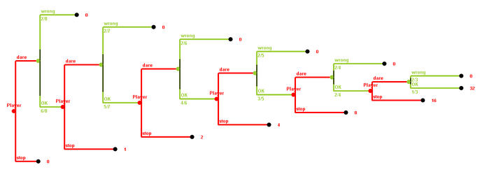
Here is the tree. At each round you have the option to dare the next question
or to stop. If you stop, an edge goes to a leaf, an end situation,
and red number written at that leaf shows how much you have won.
If you dare the next question, an edge goes to a green vertex, where
a random experiment is performed. This random experiment has
two outcomes---the answer can be correct or wrong. The probabilities for the
two oucomes are written below the green edge. If the answer was wrong, we have again
reached a leaf, a final situation, with payoff of 0. Otherwise, you are facing the decision
whether to stop or to dare the next question of the next round.

What we want to do is to assign expected payoffs to all vertices of the tree,
not just to the leaves. However, if we want to do this by beginning at the beginning
we face some problems. What is the expected payoff for the game at the very beginning?
Probably it is best to "dare" the first question. Then the payoff for the first decision
vertex is the same as the expected payoff at the first green (random) vertex.
But this expected payoff would be 2/8·0 + 6/8· the expected payoff of the
second player vertex. But this is also unknown, and so on.

The procedure demonstrated at the example above is called
backwards induction. Starting at the leaves to the right, we assign
expected payoffs to their predecessors, and the predecessors of that predecessors, and so on,
moving from right to left (backwards). Whenever we have a random vertex, we compute the expected value.
Whenever we face a decision vertex for the player, we choose the decision leading to the vertex
with the highest expected payoff (the maximum), and this maximum is also the expected payoff of our
decision vertex in question.
5 Envelopes
$10000 is distributed into 5 envelopes.
One envelope, the "bomb", remains empty.
In the basic version the player
knows how much is put into each envelope, let's say
$1000, $2000, $3000, $4000, and 0.
Then the envelopes are shuffled and in each round you, the player,
can either choose to get one of the remaining envelopes
or keep the money you have collected so far and quit.
If you ask for a new envelope,
randomly one of the remaining envelopes is selected and handed to the player.
If this envelope contains nothing (the bomb), the player you lose all
the money you collected in the previous envelopes, otherwise
you add the money to the money taken so far.
Here is an Excel analysis of the game.
How much would you "expect"
to win when you were playing the game? Would you expect to win more or less
if the $10000 were differently distributed on the envelopes,
say as $2000, $2000, $2000, $2000, and 0? What if it were distributed
as $100, $500, $2600, $7000, and 0?
What about other distributions? Would you play different then?
And what exactly does "expectation" mean?
Version b: In another version, you, the player can distribute the money into the
envelopes (using the requirement that one of them, the bomb, has to remain empty)
before starting to play.
How would you distribute the money, and how would you play?
Version c: In still another version, the distribution of the money on the
5 envelopes is not known to the player. It is just known that exactly
one envelope is empty and that the other four contain all the 10000
Dollar. How would expected value and strategy change? Would they change?
The decision tree of the original 5 Envelopes "game"
can be seen here.
Since it is so huge, and since the situations where you have drawn first $2000,
and then $3000, or where you have drawn first $3000, and then $2000 are really identical situation
for you, it is better to identify such situations and move to the digraph.
This digraph can be seen in this
Excel sheet,, where backwards induction is done automatically.
There are five envelopes, containing amounts A, B, C, D, and 0. You can change the amounts
A, B, C, D by typing in different numbers into cells B4 to B7.
Actually the random vertices are omitted, all vertices are decision vertices, they are labeled
by the bills received so far, and they are colored
black if they are final situations (with nothing to decide), red if you rather stop,
and green if you rather proceed. The expected value if proceeding is shown in the grey cell
below the situation name, and the payoff if stopping, the accumulated payoff,
is shown in the yellow cell. In each case, the payoff of that decision vertex is the maximum of both values.
Therefore the expected payoff of the original version is $3200.
Oh-No
You can play ten plays "Oh-No" here.
The player rolls a die repeatedly. After each roll, as much dollars as the die
shows are added to a heap, which initially is empty. The game ends if either
- the player decides that the heap contains enough money, takes the money in the heap,
and goes, or
- if a "1" is rolled, in which case all the money already collected in the heap
is lost.
Analysis of the "Oh-No" Game:
Note that if your sum is n so far, the expected value
if you stop is (of course) n, whereas the expected value
after the next roll of the die is
0 + (n+2)/6 + (n+3)/5 + (n+4)/6 + (n+5)/6 + (n+6)/6.
When is this value smaller than n? Just for 20 < n. Thus the best strategy
is to roll until you have 20 points. Then you stop.
The expected value, however, is smaller than 20 if using this optimal strategy.
How large is it? What changes in the "6"-version of the game,
where a "6" loses? Look at the
Excel sheet analysis.
More links
Exercises
- Consider the following variant of draw poker. Each player gets a hand of three
cards out of a 32 card deck. The ordering of the hands is straight flush (5 points),
triple (4 points), flush (3 points), pair (2 points), straight (1 point), and nothing (0 point).
Each player is allowed to exchange one card from her hand against an unknown card from the deck.
What is the optimal way to proceed if the goal is to maximize the expected points of the hand.
- We face the same situation as in the previous exercise, but a more realistic goal (if the game
is played in the usual way that the highest hand wins) is to maximize the expected value of
the percentile of the hand, where straight has percentile of 80.8 (the probability in percent
to have nothing), pair has percentile 80.8+7.26=88.065, flush has percentile of 80.8+7.26+6.77=94.839,
triple has percentile of 80.8+7.26+6.77+4.03=98.871 and straight flush finally has a percentile of
80.8+7.26+6.77+4.03+0.645=99.516=100-0.484. Would the perfect strategy change? (For simplicity we
assume that two hands of the same type, say to straights, have equal weight, also this is not the case
in reality.)


